Research: Measurements and Analysis

Research: Measurements and Analysis

Research designs are categorized in several ways, yet typically include four key, broad categories: quantitative, qualitative, mixed-method, and single-subject.

• Quantitative research

Quantitative research involves examining the relationship between variables using numerical measurements. Professional counselors use quantitative research to test hypotheses and explore descriptive or causal relationships among variables. The results of quantitative research are typically presented in a statistically significant manner, utilizing numbers and statistical analysis. Quantitative research is often distinguished from qualitative research, but can also be combined in mixed-method research designs. Here are some examples of quantitative research:

• Measuring waiting room wait times
• Conducting experimental studies comparing the effects of a placebo and an actual drug
• Performing surveys to study voter preferences

• Qualitative research

Qualitative research attempts to answer questions about how a behavior or phenomenon occurs. Data are typically represented in words rather than numbers and usually take the form of interview transcripts, field notes, pictures, video, or artifacts. The sampling is usually not randomized like that of a quantitative study, and the research can be more exploratory, meaning a hypothesis is not being tested. There is also greater subjectivity as the professional counselor plays a key role in the research. Qualitative research is useful in exploring policy or evaluating research itself. Some examples of qualitative research studies are:

• Observing and interviewing children to understand differences in the ways boys and girls play;
• Studying a subculture to understand mores;
• Case study research; and
• Policy evaluation.

• Mixed-methods research

Mixed-methods research combines quantitative and qualitative approaches, providing a comprehensive understanding beyond what each method can achieve alone. It offers several advantages, including the ability to strengthen research outcomes, apply to a broader range of inquiries, and generate more generalizable results. However, conducting mixed-methods research can be time-consuming compared to using a single method. Two common designs are:

• Concurrent design: Quantitative and qualitative data are collected simultaneously, often referred to as triangulation.
• Sequential design: Either quantitative or qualitative data is collected first. When qualitative strategies are used initially, it is exploratory; when quantitative strategies are introduced first, it is explanatory.

Some examples of mixed-methods research designs include:

• Experiment followed by qualitative data collection
• Interviews leading to instrument development
• Observing nonverbal behaviors during survey completion

• Single-subject research designs

Single-subject research designs (SSRD) measure the impact of treatment or no treatment on a single subject or group of subjects treated as a unit. This quantitative research approach is commonly used to study behavior modification and analyze behavior changes.

1. Quantitative Research Design

Quantitative research designs in counseling can be classified into two main categories: nonexperimental and experimental designs.

• Nonexperimental research designs

Nonexperimental research designs are exploratory and descriptive in nature. These designs do not involve any intervention or manipulation of variables or conditions. The primary goal of nonexperimental research is to observe and describe the properties and characteristics of a particular variable or phenomenon.

• Experimental research designs

Experimental research designs involve an intervention where a counselor manipulates variables or conditions. The objective of experimental research is to assess cause-and-effect relationships between variables. Random assignment is often a crucial component of experimental designs. These designs may involve a single group, a comparison between a treatment and control group, or a comparison between two treatment groups.

While qualitative design components can be present, single-subject research designs (SSRDs) are primarily considered as examples of quantitative research designs. SSRDs focus on measuring behavioral and/or attitudinal changes over time for an individual or a small group of individuals.

1.1. Nonexperimental Research Designs

A nonexperimental research design lacks control or manipulation of independent variables and does not involve random assignment. The four types of nonexperimental research designs are descriptive, comparative, correlational, and ex post facto designs.

• Descriptive designs involve thoroughly describing a variable at one time (simple descriptive design) or over time (longitudinal design). Simple descriptive designs are one-shot surveys that provide information about a variable. Cross-sectional designs compare different groups at the same time, while longitudinal designs track the same population or individuals over time.
• Comparative designs investigate group differences for a variable without establishing causation. They explore differences between groups but do not imply a cause-and-effect relationship. Examples include examining racial differences in mental health service utilization or gender differences in math achievement scores.
• Correlational research designs describe the relationship between two variables. Correlation coefficients are used to measure the strength and direction of the relationship. The coefficient of determination can be calculated by squaring the correlation coefficient, representing the amount of shared variance between the variables.
• Ex post facto research designs, also known as causal comparative designs, explore how an independent variable affects a dependent variable by assessing preexisting conditions that may have caused group differences. These designs examine potential causes after the data have been collected and cannot manipulate independent variables. They aim to identify associations between variables based on matched groups with different characteristics.

In counseling research, these nonexperimental designs allow for the exploration of variables, group differences, relationships, and potential causes within a given population. They provide valuable insights and understanding of various aspects related to counseling processes and outcomes.

1.2. Considerations in Experimental Research Designs

When studying the effects of an intervention, researchers should consider the three general categories of experimental designs: within-subject, between-groups, and split-plot designs.

• Within-subject designs assess changes within participants as they experience an intervention. This can involve measuring changes in a dependent variable before and after an intervention or comparing the effectiveness of multiple interventions over time within a group.
• Between-groups designs explore the effects of an intervention between two or more separate groups. Each group serves as a control or receives a distinct treatment.
• Split-plot designs assess a general intervention on the whole group while examining other treatments within smaller subgroups. This design is suitable for counseling research, such as studying the impact of a mentoring club for international students on career preparation. The subgroups may focus on different components like resume writing, job shadowing, or interviewing skills.

These experimental designs provide frameworks for investigating the effects of interventions and understanding their impact on participants in counseling research.

1.3. Experimental Research Designs

There are three main types of experimental research designs: pre-experimental, true-experimental, and quasi-experimental. The table below visually illustrates these designs. While some counselors include Single-Subject Research Designs (SSRDs) within the category of experimental designs, others consider them as a separate quantitative design.

Graphical Representations of Experimental Designs.

Pre-experimental designs
1. One-group posttest-only design	A: X → O
2. One-group pretest-posttest design	A : O → X → O
3. Nonequivalent groups posttest-only design	A : X → O
	B : n/a → O
True experimental designs
4. Randomized pretest-posttest control group design	(R) A : O → X → O(R) B : O → n/a → O
5. Randomized pretest-posttest comparison group design	(R) A : O → X → O(R) B : O → Y → O(R) C : O → Z → O
6. Randomized posttest-only control group design	(R) A : X → O(R) B : n/a → O
7. Randomized posttest-only comparison group design	(R) A : X → O(R) B : Y → O
8. Solomon four-group design	(R) A : O → X → O(R) B : O → n/a → O(R) C : n/a → X → O(R) n/a : → n/a → OA
Quasi-experimental designs
9. Nonequivalent groups pretest-posttest control group designs	A : O → X → OB : O → n/a → O
10. Nonequivalent groups pretest-posttest comparison group designs	A : O → X → OB : O → Y → OC : O → Z → O
11. Time series designsA. One-group interrupted series designB. Control group interrupted time series design	A : O → O → O → X → O → O → OA : O → O → O → X → O → O → OB : O → O → O → n/a → O → O → O

Note. A, B, and C = groups; O = observation; X, Y, Z = intervention; (R) = random assignment; n/a = control group (no intervention or observation).

Pre-experimental designs lack random assignment and therefore do not meet the criteria for true experimental designs, as they do not adequately control for internal validity threats. There are three types of pre-experimental designs:

• One-group posttest-only design: In this design, a single group receives an intervention, and the resulting change is measured. For example, the level of depression symptoms is assessed after individuals participate in a structured counseling intervention.
• One-group pretest-posttest design: This design involves evaluating a group both before and after an intervention. By comparing the pre- and post-intervention measurements, the change in the targeted variable can be examined. For instance, depression symptoms are assessed before and after individuals attend a structured counseling intervention to determine the impact on their level of depression.
• Nonequivalent groups posttest-only design: In this design, no effort is made to establish equivalent groups at the beginning of the study. One group receives the intervention while another group, serving as a control, does not receive any treatment but is assessed at the same time as the intervention group. For example, one group undergoes counseling while the other group does not receive any treatment, and the levels of depression symptoms are measured for both groups after the counseling intervention.

It is important to note that pre-experimental designs have limitations in terms of internal validity, as they do not incorporate random assignment.

True experimental designs, also called randomized experimental designs, are considered the gold standard in experimental research. They involve at least two groups for comparison and utilize random assignment, which sets them apart from quasi-experimental designs. Here are the two main types of true experimental designs:

• Randomized pretest-posttest control group design: Participants are divided into two groups, with one group serving as the control. Both groups are measured before and after an intervention to assess its effects.
• Randomized pretest-posttest comparison group design: Participants are assigned to at least two groups, and each group receives a different intervention. The effectiveness of the interventions is compared by measuring participants before and after the interventions.

• Randomized posttest-only control group design: Participants are randomly assigned to either a treatment or control group. The treatment group receives an intervention, and both groups are measured after the intervention to evaluate the outcome.
• Randomized posttest-only comparison group design: Similar to the posttest-only control group design, but involves multiple groups for comparison. Participants are randomly assigned to different groups, with each group receiving a different intervention or condition. The outcomes are measured after the interventions to compare their effects.
• Solomon four-group design: This design is a comprehensive true experimental design that combines elements of both the pretest-posttest control group design and the posttest-only control group design. It includes four randomly assigned groups:

• Group 1: Receives a pretest, intervention, and posttest.
• Group 2: Receives a pretest and posttest, but no intervention.
• Group 3: Receives an intervention and posttest, but no pretest.
• Group 4: Serves as a control and receives a posttest only, with no pretest or intervention.

Quasi-experimental designs are utilized when random assignment of participants to groups is either impossible or inappropriate. These designs are commonly employed when dealing with nested data, such as classrooms or counseling groups, or when studying naturally occurring groups like males, African Americans, or adolescents. There are two main types of quasi-experimental designs:

• Nonequivalent groups pretest-posttest control or comparison group designs: In this design, the counselor maintains the integrity of existing groups and proceeds with a pretest. Treatment is then administered to one group (in the case of a control group design) or to multiple groups (in the case of comparison group designs). Finally, a posttest is administered to all the groups to measure the outcomes.
• Time series design: This design involves repeatedly measuring variables before and after an intervention for a single group (one group interrupted time series design) or including a control group for comparison (control group interrupted time series design). In time series designs, observations are made at consistent time intervals using the same testing procedures. The treatment or intervention is implemented in a way that interrupts the baseline and is distinguishable within the research environment.

1.4. Single-Subject Research Designs

SSRDs allow for repeated measures of a target behavior over time for an individual or a select group of individuals. SSRDs are useful for counselors because they often provide concrete assessments of the effectiveness of programs for specific clients. In SSRD, A means a baseline data collection phase (without treatment), and B means a treatment data collection phase. The following are the three types of SSRDs:

• A within-series design examines the effectiveness of one intervention or program. 
• A between-series design compares the effectiveness of two or more interventions for a single variable.
• Multiple-baseline designs assess data for a particular target behavior across various individuals, environments, or behaviors. 

1.5. Descriptive Statistics

Descriptive statistics serve the purpose of organizing and summarizing data, providing a description of the data set. They are often the initial step in analyzing a data set, helping to understand how the data compare to a larger population.

After obtaining a clear understanding of the data set, the question arises: “How can we generalize our findings to the population of interest?”

This section focuses on techniques for presenting raw data sets or data distributions using tables and graphs. Additionally, it covers methods for determining typical scores within a data distribution, measures of variability, characteristics of data distributions, and the shapes they can take.

1.5.1. Presenting the Data Set

Table 8.6 provides raw-score data with the variable being number of beers consumed on average per week by each participant. The data in the table are used to demonstrate how to describe the data set.

• Frequency Distribution

A frequency distribution is a tabulation of the number of observations (or number of participants) per distinct response for a particular variable. It is presented in table format, with rows indicating each distinct response and columns presenting the frequency for which that response occurred.

The following table contains the frequency distribution for an example data presented of high school senior’s frequency of alcohol use. The first column of a frequency distribution indicates the possible data points, or it may represent intervals or clusters of data points (grouped frequency distributions). By examining the column “Cumulative Percent,” we can assess what percentage of the 30 students drank a particular amount (or provided a particular response). For example, 80% of the respondents reportedly drank seven beers or less on average per week.

Students responded to an Alcohol Use Survey. One of the items was “How many beers on average do you drink each week?” Here are the raw data for 30 respondents:

Frequency Distribution for Alcohol Consumption

Valid	Frequency	Percent	Valid Percent	Cumulative Percent
0	3	10.0	10.0	10.0
1	3	10.0	10.0	20.0
2	6	20.0	20.0	40.0
3	3	10.0	10.0	50.0
4	3	10.0	10.0	60.0
5	2	6.7	6.7	66.7
6	3	10.0	10.0	76.7
7	1	3.3	3.3	80.0
8	1	3.3	3.3	83.3
9	1	3.3	3.3	86.7
10	2	6.7	6.7	93.3
12	1	3.3	3.3	96.7
25	1	2.3	3.3	100.0
Total	30	100.0	100.0

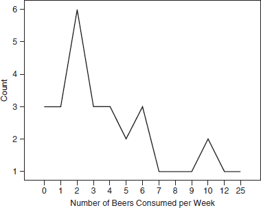
• Frequency Polygon

The frequency polygon is a line graph of the frequency distribution. The X-axis typically indicates the possible values, and the Y-axis typically represents the frequency count for each of those values. A frequency polygon is used to visually display data that are ordinal, interval, or ratio. The figure below demonstrates what a frequency polygon would look like.

Frequency polygon

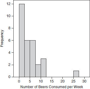
• Histogram

A histogram is a graph of connecting bars that shows the frequency of scores for a variable. Taller bars indicate greater frequency or number of responses. Histograms are used with quantitative and continuous variables (ordinal, interval, or ratio). The following figure provides an example of histogram 

Histogram

• Bar Graphs

Although it may look similar to a histogram, a bar graph displays nominal data. Each bar represents a distinct (noncontinuous) response, and the height of the bar indicates the frequency of that response. The figure below provides an example of a bar graph

Bar graph by gender of participants in a study.

1.5.2 Measures of Central Tendency

Measures of central tendency relate to the question, “What is the typical score?”. The three measures of central tendency, or three ways to assess the typical score, are the mean, median, and mode.

• The mean is the arithmetic average of a set of scores. It is computed by summing the values of all the data points and dividing by the total number of participants. An important concept in computing the mean is the presence of an outlier. An outlier is an extreme data point that distorts the mean (i.e., it inflates or deflates the typical score). 
• The median is the middlemost score when the scores are ordered from smallest to largest, or largest to smallest. When the number of scores is even, one takes the average of the two middlemost scores (i.e., interpolates them).
• The mode is the most frequently occurring score. If a data set has two most frequently occurring scores, it is said to be bimodal. If a data set has more than two frequently occurring scores, it is multimodal.

1.5.3. Variability

Variability answers the question “How dispersed are scores from a measure of central tendency?” It is the amount of spread in a distribution of scores or data points. The more dispersed the data points, the more variability for that set of data points. The three main types of variability are range, standard deviation, and variance.

• The range (R) is the most basic indicator of variability, computed by subtracting the smallest value from the largest value and adding 1 place value (e.g., in the case of whole numbers add 1, in the case of tenths add 0.1, etc.).
• The standard deviation (s, sd, and SD) is the most frequently reported indicator of variability for interval or ratio data. The standard deviation of a known population is indicated by σ Each data point is determined to be a certain number of units away from the central or average score. The larger the standard deviation, the greater the variability in scores.

• SPSS is ordinarily used to calculate the standard deviation, but the formula for standard deviation (corrected for attenuation) is ; that is, the standard deviation is the square root of the sum of squares (SS) divided by the sample size (N) − 1 (a correction for attenuation due to small sample size). The sum of squares (SS) refers to sum of the squared deviation scores and is computed by subtracting the mean from each score (deviation scores), squaring each deviation score, and adding them together [Σ(X −M)²].
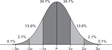
• In the normal curve, the standard deviation divides the normal distribution into approximately six parts, as displayed in the following figure.
• Variance is the final form of variability, and it is the standard deviation squared. Because variance is stated in units that are squared, standard deviation is more frequently used to explain the concept of variability.

The normal curve.

1.5.4. Skewness

Skewness pertains to the asymmetry of a distribution, where data points do not cluster evenly around the mean. In some distributions, scores tend to concentrate either towards the lower end (with more lower scores than higher scores) or the higher end (with more higher scores than lower scores). These distributions are referred to as positively skewed (skewed to the right) or negatively skewed (skewed to the left), respectively.

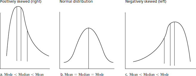
• Skewness is directly related to measures of central tendency. That is, by examining the order or sequence of values for mean, median, and mode, you can determine the degree to which your data distribution is skewed:

• Positively Skewed: Mode < Median < Mean
• Symmetrical (Normal Curve): Mean = Median = Mode
• Negatively Skewed: Mean < Median < Mode
• In SPSS output, a positive valence (+) in front of the skewness value indicates a positively skewed distribution, and a negative valence (−) in front of the skewness value indicates a negatively skewed distribution. Ordinarily, a skewness index of − 1.00 to + 1.00 indicates a nonskewed distribution.

Relationship of mean, median, and mode in normal and

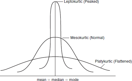
1.5.5. Kurtosis

Kurtosis is a measure that describes the shape of a data distribution, specifically its “peakedness.” It informs us about the concentration of data points within the distribution. A highly peaked distribution indicates that scores are closely clustered around the mean, with more data points in that region. Conversely, a flatter distribution suggests that scores are more dispersed from the mean, resulting in a less pronounced peak.

• The three general shapes of distributions are mesokurtic (normal curve), leptokurtic (tall and thin), and platykurtic (flat and wide).
• Kurtosis is represented by numeric values, which can be easily derived from SPSS. A mesokurtic, or normal, distribution has a kurtosis value of 0 (technically from − 1.00 to + 1.00); a leptokurtic distribution, demonstrating more peakedness, has a positive kurtosis value (i.e., > 1.00); and a platykurtic distribution, being flatter than the normal distribution, has a negative kurtosis value (i.e., < − 1.00).

Examples of kurtosis.

1.6. Inferential Statistics

Inferential statistics is a statistical approach that goes beyond the data itself and aims to make conclusions about a larger population of interest. It differs from descriptive statistics, which simply describe the data. By using inferential statistics, researchers can make inferences about populations based on the probability of certain differences, without needing to test every individual within the population.

• Statistical tests play a crucial role in inferential statistics. The choice of a specific test depends on various factors, including the research question, the types of groups involved, the number of variables, the scale of measurement, and the ability to meet certain statistical assumptions. These assumptions include the normal distribution of the dependent variable, random sampling or assignment, and the use of interval or ratio scales of measurement.
• When the statistical assumptions are met, parametric statistics are used. If the assumptions are not met, nonparametric statistics are employed. However, researchers often still use parametric statistics even when the assumptions are violated because they tend to be robust.
• Degrees of freedom is an important concept in inferential statistics. It refers to the number of scores or categories of a variable that can vary freely. Degrees of freedom are integral to most inferential statistics formulas and are calculated based on the chosen statistical test. They are determined by subtracting the number of parameters from the total number of scores or categories (typically represented as n – 1). Having more degrees of freedom provides greater confidence that the sample is representative of the population.

1.6.1. Correlation

A correlation coefficient describes the relationship between two variables, indicating if a relationship exists, its direction, and strength.

• The absolute value of the correlation represents its strength (e.g., -0.87, -0.63).
• The sign (+ or -) shows the direction: positive when variables move together, negative when they move in opposite directions.
• Correlation values range from -1.00 to +1.00, often measured with the Pearson product-moment correlation coefficient (Pearson r). +1.00 indicates a perfect positive relationship, -1.00 a perfect negative relationship. Other coefficients include Spearman r (rank-order variables), biserial correlation (continuous and dichotomous), and point biserial correlation (continuous and true dichotomous).
• Correlations reveal association, not causation.
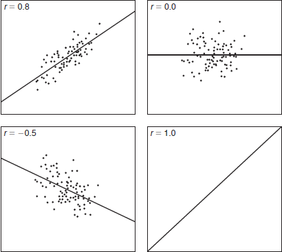
• Scatterplots illustrate correlations. Spurious correlations overstate or understate the relationship, caused by shared variables or unmeasured factors.
• Unreliable measures can mislead correlations, underestimating the relationship (attenuation).
• Inaccurate relationships can result from limited sample representativeness.
• Decimals in correlations are not percentages. Squaring correlation values provides the coefficient of determination (r^2), representing the shared variance between variables.

Examples of scatterplots.

1.6.2. Regression

Prediction studies, also known as regression studies, build upon correlational research by allowing professional counselors to make predictions based on high correlations between variables. Although they do not provide explanations like experimental designs, they offer opportunities for outcome predictions. There are three types of regression:

• Bivariate regression: Examines how scores on an independent variable (predictor variable) predict scores on the dependent variable (criterion variable).
• Multiple regression: Involves multiple predictor variables, each with a weighted contribution (beta weights) in a regression equation. The more predictor variables used, the stronger the prediction can be.
• Logistic regression: Used when the dependent variable is dichotomous. This form of regression can be similar to bivariate or multiple regression.

1.6.3 Parametric Statistics

Parametric statistics are utilized when the necessary statistical assumptions are met. Within this category, several common tests can be employed, including:

• T-test

Compares the means of two groups for a single variable. Independent t-tests are used for comparing two independent groups, such as gender differences in achievement. Dependent t-tests (repeated measures t-tests) involve paired or matched groups, or the same group tested twice.

• Analysis of Variance (ANOVA)

Examines differences among three or more groups or levels of an independent variable. ANOVA extends the t-test and provides an F ratio to determine if group means are statistically different. Post hoc analysis allows for comparisons between specific group pairs after establishing significant main effects.

• Factorial ANOVA

Used when multiple independent variables are present, allowing for the examination of main effects and interaction effects. Interaction effects reveal significant differences among groups across two or more independent variables. Post hoc analysis helps determine the direction and existence of these interactions.

• Analysis of Covariance (ANCOVA)

Incorporates an independent variable as a covariate to control and adjust for its influence on the relationship between other independent variables and the dependent variable. Conducting a factorial ANOVA is preferable if the covariate is of primary interest.

• Multivariate Analysis of Variance (MANOVA)

Similar to ANOVA but involves multiple dependent variables, enabling the examination of differences among groups across multiple outcome variables.

• Multivariate Analysis of Covariance (MANCOVA)

Similar to ANCOVA but encompasses multiple dependent variables, allowing for the control of covariates when examining differences among groups.

These parametric statistical tests are valuable tools for analyzing data in a variety of research contexts.

1.6.4. Nonparametric Statistics

Nonparametric statistics are employed by professional counselors when they can make limited assumptions about the distribution of scores in the population of interest. These statistics are particularly useful for nominal or ordinal data and situations where interval or ratio data do not follow a normal distribution, such as when the data is skewed. Several commonly used nonparametric statistics include:

• Chi-square test

Used with two or more categorical or nominal variables, where each variable contains at least two categories. All scores must be independent—that is, the same person cannot be in multiple categories of the same variable. The professional counselor forms the categories and then counts the frequency of observations or categories. Then, the reported (or observed) frequencies are compared statistically with theoretical or expected frequencies.

• Mann-Whitney U test

Analogous to a parametric independent t-test, except the Mann-Whitney U test uses ordinal data instead of interval or ratio data. This test compares the ranks from two groups.

• Kolmogorov-Smirnov Z procedure

Similar to the Mann-Whitney U test but more appropriate to use when samples are smaller than 25 participants.

• Kruskal-Wallis test

Analogous to an ANOVA. This test is an extension of the Mann-Whitney U test when there are three or more groups per independent variable.

• Wilcoxon’s signed-ranks test

Equivalent to a dependent t-test. This test involves ranking the amount and direction of change for each pair of scores. For example, this test would be appropriate for assessing changes in perceived level of competency before and after a training program.

• Friedman’s rank test

Similar to Wilcoxon’s signed-ranks test in that it is designed for repeated measures. In addition, it may be used with more than two comparison groups.

1.6.5. Factor Analysis

Factor analysis is used to condense a large number of variables into a smaller number of factors that explain the covariation among the variables. Factors are hypothetical constructs that account for the shared variance among the variables. There are two forms of factor analysis: exploratory factor analysis (EFA) and confirmatory factor analysis (CFA).

• In EFA, potential models or factor structures are examined to categorize the variables. It involves two steps: factor extraction and factor rotation. Factor extraction is like mining for precious metals, where the goal is to extract the metals (factors) that share commonalities among variables. Factor rotation helps interpret the factors by changing the reference point for variables without altering their relationships. Common types of factor extractions include principal axis factoring, principal components analysis, and maximum likelihood method. Factor rotation can be orthogonal (uncorrelated factors) or oblique (correlated factors).
• CFA confirms the results of EFA. The most common method is the maximum likelihood method. After obtaining a factor solution, the overall fit of the model to the data is assessed using fit indices such as chi-square statistic, Tucker-Lewis Index, comparative fit index, standardized root mean squared residual, and root mean squared error of approximation.

1.6.6. Meta-Analysis

Meta-analysis is a method to combine and synthesize results from multiple studies on a specific outcome variable. It helps determine the overall average effect and addresses discrepancies or contradictions in individual studies. In counseling research, meta-analysis is widely used to examine the effectiveness of counseling interventions.

Steps in conducting a meta-analysis include establishing inclusion criteria, locating relevant studies, coding independent variables, calculating effect sizes for each outcome variable, and comparing and combining effect sizes across studies.

• Establish criteria for including a study based on operational definitions (e.g., psychotherapy and counseling).
• Locate empirical studies based on criteria. Include dissertations and theses as appropriate.
• Consider and code variables that could be independent variables (e.g., length of treatment, counselor training, rigor of research design).
• The dependent variable in a meta-analysis is the effect size (i.e., a measure of the strength of the relationship between two variables in a population) of the outcome. Calculate an effect size on any outcome variable in the study. Thus, there may be several effect sizes per study.
• Effect sizes are compared and combined across studies and grouped according to independent variables of interest.

2. Qualitative Research Design

Qualitative research explores processes and the meaning individuals attribute to phenomena. It is often used when little research is available or when counselors want to understand a topic from a specific group’s perspective. Counselors conducting qualitative research should consider the following:

• How do individuals describe the phenomenon within their context?
• What is the process or sequence of the phenomenon?
• How can individuals contribute as experts on the phenomenon?
• How can individuals be involved in the research team?
• How do data contribute to the evolving theory or detailed understanding of the phenomenon?
• How does the researcher’s participation affect data collection and analysis?
• How can validity be maximized in the study? To what extent should participants’ narratives be included in the findings?

Qualitative research has additional characteristics, which are outlined in the table below. The terms used in the table will be defined in subsequent sections.

This section describes research traditions, sampling methods, data collection methods, data management and analysis strategies, and strategies for establishing trustworthiness.

Characteristics of Qualitative Research.

Study of issues in depth and detailContextualDiscovery-oriented approachHow social experience is created and given meaningThick descriptionFieldworkResearch design constantly evolvingInductive analysisResearcher as instrumentParticipants as experts/partners in researchParticipant observationInterviewingDocument analysisPurposeful samplingReflexivityThemes vs. numbersTrustworthiness

Note. Summarized from Maxwell and Hays and Singh

2.1 Qualitative Research Traditions

Qualitative research is guided by various research traditions that shape decisions related to sampling, data collection, and data analysis. Here are summaries of the seven major research traditions covered in this section:

• Case study

This tradition involves studying a distinct system, event, process, or individuals in-depth. Active participation of those involved in the case is integral to data collection.

• Phenomenology

Phenomenology aims to understand the meaning and essence of participants’ lived experiences, focusing on individual and collective human experiences for different phenomena.

• Grounded theory

This influential approach aims to generate theory grounded in participants’ perspectives and data. It is an inductive approach that often explains processes or actions related to a specific topic.

• Consensual qualitative research (CQR)

CQR combines elements of phenomenology and grounded theory, involving knowledgeable participants and emphasizing consensus in interpretations. Power dynamics and rigorous methods play a significant role in this approach.

• Ethnography

Ethnography focuses on describing and interpreting the culture of a group or system, often using participant observation to explore socialization processes. It provides insights into how a community addresses certain issues, such as mental health concerns.

• Biography

Biography aims to uncover the personal meanings individuals assign to their social experiences. Stories are gathered and explored in the context of broader social or historical aspects. Biographical methods include life history and oral history.

• Participatory action research (PAR)

PAR emphasizes participant and researcher transformation as a result of qualitative inquiry. It focuses on achieving emancipation and transformation, involving collaboration between the researcher and stakeholders to address issues and bring about positive change.

These research traditions offer unique approaches to qualitative inquiry, each suited for different research purposes and contexts.

2.2. Purposive Sampling

Purposive sampling, also known as purposeful sampling, aims to select information-rich cases that provide in-depth understanding of a phenomenon. Counselors typically seek saturation, where new data no longer contradict previously collected findings. There are approximately 15 types of purposive sampling methods.

• Convenience sampling: Sampling based on availability or accessibility, although it is considered less desirable and less reliable.
• Maximum variation sampling: Sampling a diverse group to identify core patterns and individual perspectives based on unique participant characteristics.
• Homogenous sampling: Selecting participants from a specific subgroup who share theoretically similar experiences.
• Stratified purposeful sampling: Identifying important variables and sampling subgroups that isolate each variable, also known as “samples within samples.”
• Purposeful random sampling: Identifying a sample and randomly selecting participants from that sample.
• Comprehensive sampling: Sampling all individuals within a system, particularly useful when the case has few participants.
• Typical case sampling: Selecting participants who represent the average or typical experience of a phenomenon.
• Intensity sampling: Identifying participants with intense (but not extreme) experiences of a phenomenon.
• Critical case sampling: Sampling participants with intense and irregular experiences to illustrate a point and gain extensive knowledge.
• Extreme or deviant sampling: Selecting participants with the most positive and negative experiences to explore both ends of a continuum.
• Snowball, chain, or network sampling: Obtaining recommendations from earlier participants to expand the pool of participants, commonly used when sample recruitment is challenging.
• Criterion sampling: Developing specific criteria and selecting all cases that meet the criteria.
• Opportunistic or emergent sampling: Seizing unexpected opportunities and modifying the research design to include particular individuals in the sample.
• Theoretical sampling: Sampling individuals who contribute relevant information to the evolving theory.
• Confirming and disconfirming case sampling: Including cases that confirm and deepen the evolving theory, as well as those that present exceptions or potentially challenge elements of the theory. This is often done as part of theoretical sampling.

2.3. Qualitative Data Collection Methods

Qualitative data collection methods can be categorized into three main types: interviews, observations, and unobtrusive methods such as document analysis and photography. It is recommended to employ multiple methods to enhance the richness of qualitative research. The table below highlights the potential strengths and limitations of each method.

Qualitative Data Collection Methods.

Method	Strengths	Limitations
Interviews	Can be adapted to include one individual or several individuals at one timeAllows participants to describe their perspectives directlyEncourages interaction between counselor and participantMay be cost effective	May differ in the degree of structure as well as format and thus not provide similar amounts of data across participantsDepending on the type of interview, possible limit to number of questions asked
Observations	Allows researcher to capture the context in which a phenomenon is occurringAdds depth to qualitative data analysis	Poorly established observation rubrics possibly leading to invalid observationsDifficult to focus on several aspects of an observation at one time
Unobtrusive methods	Can guide future data collection methodsAllow for permanence and density of dataCorroborate findings from other data sources	Some contextual information possibly missing from the source

• Qualitative Interviewing

Interviews can be categorized into unstructured, semi-structured, and structured types, varying in their level of structure. Unstructured interviews have no predetermined questions, while semi-structured interviews follow a preset protocol with some flexibility, and structured interviews have a fixed set of questions.

• Interviews can be conducted with individuals or in focus groups. Focus groups typically consist of 6 to 12 members and provide collective insights on a specific issue. Individual interviews are suitable for sensitive topics, while focus groups facilitate understanding of social interactions. It’s important to note that these two interview formats may yield different types of data.
• Observational Methods

Qualitative observations aim to provide a detailed description of the setting or context where a phenomenon occurs. Counselors engage in fieldwork and take notes (“memoing”) to analyze the content and process of the setting. Observation rubrics aligned with the research question help focus on specific aspects of the setting.

• Observation can be positioned along a continuum, ranging from minimal interaction with those observed to full participation as a group member. Participant observation is the common role for counselors conducting observations, with varying degrees of observation and participation.

The continuum of participant observation.

• Unobtrusive Methods

Unobtrusive data collection methods typically do not involve direct interactions with participants. Examples of data collection methods include collecting photographs, videos, documents (e.g., diaries, letters, newspapers, and scrapbooks), archival data, and artifacts. 

2.4. Qualitative Data Management and Analysis

In qualitative research, effective data management strategies are crucial due to the large amount of data involved. Contact summary sheets and document summary forms are useful tools for organizing data. Contact summary sheets provide a snapshot of specific contacts, including details such as time, date, setting, participant information, and key themes. Document summary forms are attached to unobtrusive data sources like newsletters or artifacts.

• Data displays, such as tables or interconnected node figures, are commonly used for data analysis and management. They can be created for individual participants (within-case displays) or the entire sample (cross-case displays).
• Inductive analysis is an important approach in qualitative data analysis, where keywords and potential themes emerge from the data without predetermined theories.
• While there are various ways to analyze qualitative data, a generic set of steps includes writing memos, constructing an initial summary, organizing and segmenting the text, coding the data, searching for themes and patterns, identifying main themes, describing them in detail, and exploring relationships among themes.

2.5. Trustworthiness

To establish the robustness of a qualitative study, it is essential to demonstrate trustworthiness by providing evidence of validity and reliability. Trustworthiness refers to the credibility and believability of the findings, ensuring that others can trust the data collection and analysis methods as well as the results.

• Four key components of trustworthiness are credibility, transferability, dependability, and confirmability. Credibility focuses on the accuracy and faithfulness of the findings, ensuring that they truly represent the study. Transferability examines the extent to which the findings can be applied to other contexts or participants, similar to generalizability in quantitative research.

Dependability relates to the consistency of the results over time and among researchers, assessing whether other counselors would obtain similar findings with the same data. Confirmability emphasizes the authentic reflection of participants’ perspectives, ensuring that counselors’ biases and assumptions have been controlled for. The table below provides strategies for maximizing these four components of trustworthiness.

Strategies for Trustworthiness

Prolonged engagement	Focus on scope of context for an extended time frame to learn about the overall culture and phenomenon.
Persistent observation	Focus on depth of context to ascertain important details and characteristics related to a research question.
Triangulation	Test for consistency and inconsistency of data by using multiple participants, data sources, researchers, or theories.
Peer debriefing	Check counselor’s biases and findings with those outside of the study.
Member checking	Consult participants to verify the truth of the findings.
Negative case analysis	Look for inconsistencies and data that might refute preliminary findings.
Referential adequacy	Check findings against archived data collected at various points of the study.
Thick description	Describe in significant detail data collection and analysis procedures.
Auditing	Select an individual with no interest in the specific results of the study to review documents and proceedings (audit trail) for accuracy of interpretations.
Reflexive journal	Memo about reflections surrounding a qualitative inquiry to assist in minimizing the influence of counselor bias in data collection, analysis, and reporting.